

A pricing curve (the technical term is a demand curve) is a simple chart with price on the vertical axis and quantity purchased on the horizontal axis. When price goes up, people buy less. That single downward-sloping line carries a direct money implication: before you absorb any price increase, check whether a substitute exists, because the shape of the curve tells you how much your spending will actually change.
Two frameworks ground everything in this guide:
- The Slutsky decomposition from the Federal Reserve Bank of Minneapolis explains how every price change splits into two forces: a substitution effect (swap to a cheaper option) and an income effect (you feel poorer and cut back overall).
- MIT’s Principles of Microeconomics lecture notes supply the elasticity formula and curve definitions used throughout.
Key Takeaways
Understanding the demand curve gives you a practical framework for every price change you face: identify your sensitivity, find substitutes, and protect essentials before cutting anything else.
| Point | Details |
|---|---|
| Demand curves slope down | Price on the vertical axis, quantity on the horizontal; higher prices mean less purchased. |
| Movement vs. shift | A price change moves you along the curve; an income or preference change shifts the whole curve. |
| Substitution and income effects | Every price hike triggers both; for normal goods, both push consumption down together. |
| Elasticity guides your response | Use ε = % change in quantity ÷ % change in price; elastic goods invite substitution, inelastic ones need structural fixes. |
| Protect essentials first | Trim discretionary spending before emergency savings when essential prices rise. |
Table of Contents
- What does a pricing curve actually show?
- Moving along the curve vs. shifting the curve
- How substitution and income effects shape your choices
- How to measure price sensitivity with elasticity
- How sellers use curves to set prices and what that means for you
- Practical steps to take when prices change
- A worked household example: gasoline
- Savings Grove’s perspective on demand-curve thinking
- Sources
What does a pricing curve actually show?
A demand curve graphs the relationship between price and quantity demanded, and according to OpenStax, most demand curves slope downward. That slope reflects the law of demand: as price rises, quantity demanded falls, all else equal. The phrase “all else equal” is the ceteris paribus assumption — it means you are only changing price, nothing else.
Before you can sketch a curve, you need a demand schedule, which is simply a table pairing prices with the quantities people buy at each price. The University of Minnesota’s open microeconomics text describes it as the practical starting point for any demand analysis.
Sample demand schedule — generic household good:
To sketch the curve, put price on the vertical (Y) axis and quantity on the horizontal (X) axis, then plot each row as a point and connect them. The resulting line slopes down and to the right.
A few things worth knowing about curve shapes:
- Steep curves signal inelastic demand (price changes barely affect quantity).
- Flat curves signal elastic demand (small price changes cause large quantity swings).
- Curves for necessities like insulin tend to be steep; curves for discretionary goods like restaurant meals tend to be flat.
Moving along the curve vs. shifting the curve
These two concepts trip up a lot of readers, and the difference matters for your budget.
Moving along the curve happens when only the price changes. Your preferences, income, and everything else stay the same. Gasoline prices spike in summer, and you drive a little less — that is a movement along your existing demand curve.
Shifting the curve happens when something other than price changes your underlying desire or ability to buy. The curve itself moves left (less demand at every price) or right (more demand at every price). The Federal Reserve Bank of Minneapolis notes that recognizing this distinction prevents you from misreading a short-term price response as a permanent preference change.
Non-price factors that shift your personal demand curve:
- Income changes: A pay cut shifts your demand for restaurant meals left.
- Tastes and preferences: Discovering a new coffee brand shifts your demand for your old brand left.
- Prices of related goods: A big drop in streaming subscription prices shifts your demand for cable TV left.
- Expectations: Expecting a price hike next month shifts your demand right today.
- Population or household size: Adding a family member shifts demand for groceries right.
The remote-work boom is a clear real-world example. When millions of Americans stopped commuting in 2020, demand for gasoline shifted left — not because gas got more expensive, but because the underlying need changed.
How substitution and income effects shape your choices
When a price rises, two things happen to you simultaneously, and the Slutsky decomposition is the standard framework economists use to separate them.
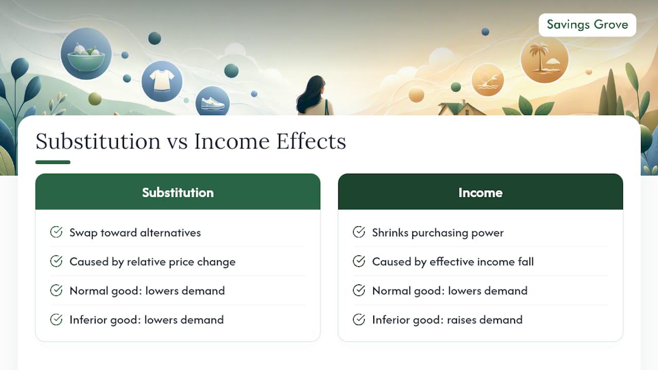
The substitution effect is straightforward: the good that got more expensive is now relatively pricier compared to alternatives, so you swap toward those alternatives. The income effect is subtler: the price increase effectively shrinks your purchasing power, so you feel poorer and may cut back on spending broadly.
Say coffee prices rise sharply. The substitution effect nudges you toward tea. The income effect means your grocery budget stretches less far, so you might also buy fewer snacks overall. For a normal good like coffee, both effects push consumption down — they reinforce each other.
The edge case is an inferior good, something you buy more of when your income falls (think store-brand pasta). If its price rises, the substitution effect still pushes you away from it, but the income effect pushes you toward it because you feel poorer. As Pindyck and Rubinfeld explain, these two effects can work in opposite directions, which is why budgeting for inferior goods gets complicated.
Pro Tip: When a price hike hits, ask yourself two questions: “What can I swap to?” (substitution) and “Does this change how much I can spend on everything else?” (income). Answering both gives you a complete picture of your response options.
How to measure price sensitivity with elasticity
Price elasticity of demand tells you how strongly quantity demanded responds to a price change. The formula, drawn from MIT OCW, is:
ε = (% change in quantity demanded) ÷ (% change in price)
Interpretation rules:
- |ε| > 1 (elastic): Quantity drops more than price rose. A 10% price increase cuts quantity by more than 10%. Total spending on that good falls.
- |ε| = 1 (unitary): Quantity drops exactly as much as price rose. Total spending stays the same.
- |ε| < 1 (inelastic): Quantity drops less than price rose. A 10% price increase cuts quantity by less than 10%. Total spending on that good rises.
Your total spending stays roughly the same. Demand is inelastic, and your monthly spending on the gym actually rises.
Elasticity varies along a single curve. The same product can be elastic at high prices and inelastic at low prices, so a quick estimate should factor in where you currently sit on the price range.
Quick heuristics for estimating elasticity without formal data:
- Necessities with few substitutes (prescription drugs, utilities): inelastic.
- Luxuries or goods with many alternatives (streaming services, brand-name snacks): elastic.
- To estimate informally, track your own purchases at two different price points over a month, then plug the percentages into the formula above.
How sellers use curves to set prices and what that means for you
Sellers build their pricing strategy around the same demand curve you are reading. A firm facing inelastic demand can raise prices and collect more revenue — consumers have few alternatives and keep buying. A firm facing elastic demand risks a sharp sales drop if it raises prices, so it competes on price instead.
OpenStax explains that a market reaches equilibrium where quantity demanded equals quantity supplied. Prices above equilibrium create a surplus (too much product, prices fall). Prices below equilibrium create a shortage (too little product, prices spike). For you as a consumer:
- A surplus often means discounts are coming — a good time to stock up on non-perishables.
- A shortage signals temporary price spikes; waiting a few weeks can save money if the good is not urgent.
- When a seller raises prices on an inelastic good (think cable internet in areas with one provider), your best response is a long-term structural change: negotiate, bundle, or find a substitute service.
Practical steps to take when prices change
Use this checklist whenever a price increase hits your budget:
- Estimate elasticity. Is this a necessity with few substitutes, or a discretionary good? Inelastic goods need a structural fix; elastic goods just need a substitute.
- List your substitutes. Write down two or three alternatives at lower price points. Check how to cut household expenses quickly for category-specific ideas.
- Calculate the monthly budget impact. Multiply the price increase by your typical monthly quantity. Even a small per-gallon gas increase can add a noticeable amount per month for an average driver.
- Decide: substitute, absorb, or restructure. Substitute when elastic alternatives exist. Absorb when the good is a true necessity and no substitute is available. Restructure (renegotiate, downgrade, or eliminate) when the good is discretionary.
- Protect essentials first. If rising essential prices force cuts, trim discretionary spending before touching emergency savings. Savings Grove’s guide on discretionary expenses helps you classify spending quickly.
Pro Tip: Run a two-week substitution test before committing. Switch to the cheaper alternative for 14 days and track satisfaction and cost. If both hold up, make the switch permanent.
For readers on tighter budgets, the money tips for low-income Americans guide at Savings Grove offers prioritized actions when essential prices rise and income is constrained.
A worked household example: gasoline
Here is how demand-curve thinking plays out at the pump. The table below shows a simplified household gasoline demand schedule with descending quantities as price increases, illustrating the inverse relationship between price and quantity demanded.
Scenario: Price rises from a lower to a higher level per gallon.
- Old spending: Price times old quantity.
- New spending at same quantity: Higher price times old quantity, showing increased spending.
- Adjusted quantity: The household cuts quantity demanded. New spending is close to the old spending level.
- Net result: By reducing quantity, the household nearly holds its fuel spending flat.
The quantity reduction reflects both effects. The substitution effect drives combining errands, carpooling, or cutting leisure drives. The income effect means the household also feels the budget squeeze and may trim other spending.
Realistic limits: If you commute 30 miles each way with no public transit option, cutting quantity is harder. In that case, the income effect dominates and you need to find savings elsewhere in the budget.

Savings Grove’s perspective on demand-curve thinking
What strikes me most about demand-curve thinking is how rarely consumers apply it consciously, even though they act on it every day. When you switch from name-brand cereal to store-brand after a price hike, you are running the substitution effect in real time. Naming it just makes you faster and more deliberate.
The bigger opportunity is elasticity awareness. Most people treat every price increase as equally painful. They are not. Treating them the same leads to cutting the wrong things.
At Savings Grove, three recommendations come up consistently when prices move: first, identify a substitute and test it before committing; second, build a short-term budget buffer of one to two months of the affected expense so a spike does not force a rushed decision; third, check whether a better deal already exists. Prices change, but so do offers, and a quick comparison often finds savings without any lifestyle change at all.
Sources
- The Mechanics of Demand | Federal Reserve Bank of Minneapolis
- 14.01 F23 Lecture Summary 4: Demand Curves | MIT OCW
- Demand, supply, and equilibrium in markets for goods and services | OpenStax
- Open Principles of Microeconomics - 3. Demand and Supply | University of Minnesota
- Pindyck & Rubinfeld — Chapter on consumer response to price changes (excerpt) | SFU
This article is general information, not a substitute for advice from a qualified financial advisor. Consult a qualified financial professional about your own circumstances before acting on anything here.